Code
library(keras)
dataset = dataset_boston_housing()
c(c(train_data, train_targets),c(test_data, test_targets)) %<-% datasetHere, we train a network to predict median housing prices of 1970s Boston !
Lets see the fight between Multiple Linear Regression and Neural Networks.

The Boston Housing dataset contains of 13 Covariates. Our aim is to predict the median price of homes in the given Boston suburb back in the mid-1970s. You can see the data library for a description of the dataset.
library(keras)
dataset = dataset_boston_housing()
c(c(train_data, train_targets),c(test_data, test_targets)) %<-% datasetThe Train-Test split ends up giving us 404 training samples and 102 for testing; each with 13 numerical categories. The target variables is the Median Values of Owner-occupied Homes, in 1000s of Dollars. The prices are typically between $10,000 and $50,000 - if that sounds cheap, remember that this was the mid-1970s, and these prices aren’t adjusted for inflation.
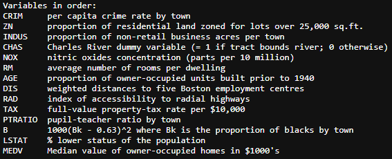
Let’s look at the distribution of the variables we have.
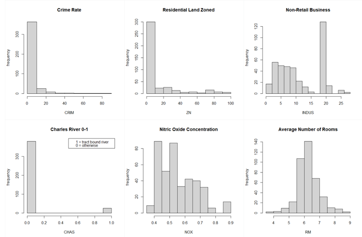
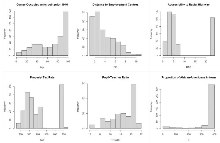
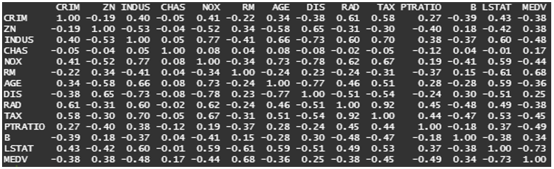
From the above graphs, we can see that a few variables like Crime Rate, Residential Land Zone & Distance to Employment Centres are positively skewed whereas variables like Pupil-Teacher Ratio, Proportion of African-Americans are negatively skewed. Based on the correlation plot, there is high correlation of Median Income with LSTAT (negative) & RM (positive).
Before we move on, we must check the range of the variables we deal with.
summary(dataset$train$x)| Variable | Variable | Minimum | Maximum |
|---|---|---|---|
| V1 | CRIM | 0.00632 | 88.976 |
| V2 | ZN | 0.00 | 100.00 |
| V3 | INDUS | 0.46 | 27.74 |
| V4 | CHAS | 0.00 | 1.00 |
| V5 | NOX | 0.385 | 0.871 |
| V6 | RM | 3.561 | 8.725 |
| V7 | AGE | 2.90 | 100.00 |
| V8 | DIS | 1.130 | 10.71 |
| V9 | RAD | 1.00 | 24.00 |
| V10 | TAX | 188.0 | 711.0 |
| V11 | PTRATIO | 12.60 | 22.00 |
| V12 | B | 0.32 | 396.90 |
| V13 | LSTAT | 1.73 | 37.97 |
| V14 | MEDV | 5.00 | 50.00 |
As we can see all the variables have very different range. So, we need to scale them! Scaling ensures that all the variables are within the same range. This becomes an important step to ensure that unfair weigthage is not given to variables with high numerical values and units.
To scale, we centre each variable around it’s average value. This is called Normalisation.
mean = apply(train_data, 2, mean) # average of all variables
sd = apply(train_data, 2, sd)     # standard deviation of all variables

train_data = scale(train_data, center = mean, scale = sd)
test_data = scale(test_data, center = mean, scale = sd)Before we jump into Deep learning, we must explore the basic Multiple Linear Regression models to set a benchmark for the DL model to outperform.
train_data = as.data.frame(train_data)
test_data = as.data.frame(test_data)
round(cor(train_data$V13, train_data[,-13]),3)
# V1 V2 V3 V4 V5 V6 V7 V8 V9 V10 V11 V12
#0.434 -0.415 0.603 -0.011 0.593 -0.611 0.591 -0.507 0.49 0.535 0.366 -0.376
library(psych)
corPlot(as.data.frame(train_data))
x = train_data[,-13]
y = train_data[,13]
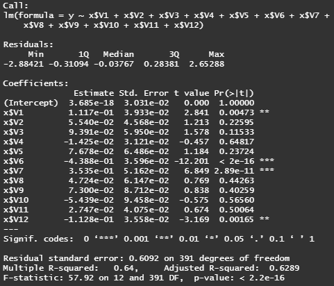
fit = lm(y~x$V1+x$V2+x$V3+x$V4+x$V5+x$V6+x$V7+x$V8+x$V9+x$V10+x$V11+x$V12)
summary(fit)
# as suspected, only variables v2, v6, v7, v12 are significant variables
# i.e. ZN (proportion of residential zone), RM (average number of rooms),
# AGE (owner-occupied houses built prior 1940), B (proportion of African-Americans)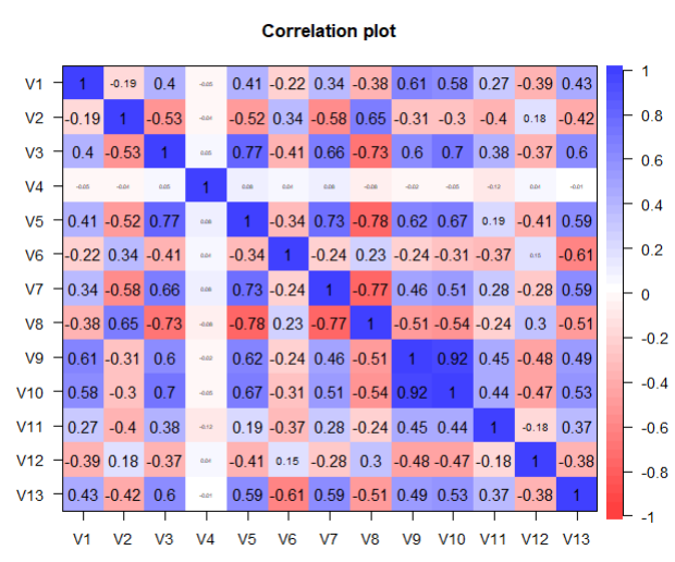
step(lm(y~x$V1+x$V2+x$V3+x$V4+x$V5+x$V6+x$V7+x$V8+x$V9+x$V10+x$V11+x$V12),
     direction = "backward")
# best model : y ~ v1 +v3 +v6 + v7 + v12

best.fit = lm(y ~ x$V1 + x$V3 + x$V6 + x$V7 + x$V12)
summary(best.fit)
# fitted regression equation
# y = 7.498e-20 + 0.132*v1  + 0.1*v3 - 0.441*v6 + 0.337*v7 - 0.129*v12

# Adjusted R-squared = 63.51%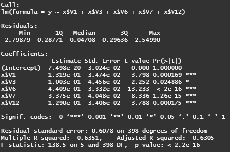
result = 7.498e-20 + 0.132*test_data$V1  + 0.1*test_data$V3
       - 0.441*test_data$V6 + 0.337*test_data$V7 - 0.129*test_data$V12

cor(result, test_data$V13) # correlation = 0.8602979

library(Metrics)
mae(test_data$V13, result) # MAE = 0.363312

library(car)
avPlots(best.fit, main = "")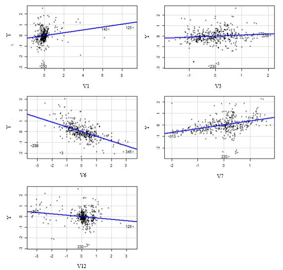
The Multiple Linear Regression Model used worked with the following Covariates :
It achieves a correlation with test values of 86% and a MAE = 0.3633 i.e. we’re approximately off by $3633 on average.
We have a small dataset, so we will use a small model to avoid overfitting. To call this model frequently - we code it as a function.
build_model <- function() {
  # network structure
  model <- keras_model_sequential() %>%
    layer_dense(units = 64, activation = "relu",
                input_shape = dim(train_data)[[2]]) %>%
    layer_dense(units = 64, activation = "relu") %>%
    layer_dense(units = 1)
  # compile
  model %>% compile(optimizer = "rmsprop",loss = "mse",metrics = c("mae"))
}
1st Layer has 64 neurons/ hidden units with a ReLU Activation. It is densely connected to the 2nd layer which also has 64 neurons and ReLU Activation.
Last Layer - A single unit with no activation so that the last layer will be a linear. This is typical set-up for scalar regression. Applying an activation function would constrain the range the output can take, for e.g. applying sigmoid activation function to the last layer, the network could only learn to predict values between 0 and 1.
For Loss Function, we use MSE i.e. Mean Squared Error = (Actual-Predicted)^2
We set metrics = c(“mae”) which allows R to keep track of Mean Absolute error = ||actual-predicted||. For example, if MAE = 0.5 it implies that we are off by $500 on average.
As we have a small dataset - the validation sample will be even smaller - the validation accuracy will highly be sensitive to the data-points selected for validation. This sensitivity will cause a high variance - making it difficult to have a refined model. Solution? We use ‘k-fold cross-validation’ where we split the sample into ’k’ partitions.
We make ‘k’ identical models - we use 1 split for validation and remaining ‘k-1’ splits for training. Each of these models give us a validation score - the final validation score is the average of all these scores.
k <- 4 # 4 models
indices <- sample(1:nrow(train_data))
# we simulate random values which we use as index to pick random training samples
folds <- cut(indices, breaks = k, labels = FALSE)
# here we divide the sample into 'k' folds

num_epochs <- 500
all_mae_histories <- NULL
for (i in 1:k) {
  cat("processing fold #", i, "\n")
  # (1) prepares the validation data from k partition
  val_indices <- which(folds == i, arr.ind = TRUE)
  val_data <- train_data[val_indices,]
  val_targets <- train_targets[val_indices]
  # (2) prepares the training data from all other partitions
  partial_train_data <- train_data[-val_indices,]
  partial_train_targets <- train_targets[-val_indices]
  # (3) builds the keras model - already compiled
  model <- build_model()
  # (4) trains the model (in silent mode, verbose=0)
  history <- model %>%
    fit(partial_train_data, partial_train_targets,
        validation_data = list(val_data, val_targets),
        epochs = num_epochs, batch_size = 1, verbose = 0)
  mae_history <- history$metrics$val_mae
  all_mae_histories <- rbind(all_mae_histories, mae_history)
}
# compute the average of the per-epoch MAE scores for all folds
average_mae_history <- data.frame(epoch = seq(1:ncol(all_mae_histories)),
                                  validation_mae = apply(all_mae_histories,
                                                         2, mean))

library(ggplot2)
ggplot(average_mae_history, aes(x=epoch, y=validation_mae))+geom_line()
# It may be a bit hard to see the plot due to scaling
# issues and relatively high variance (as mentioned above)
ggplot(average_mae_history, aes(x=epoch, y=validation_mae))+geom_smooth()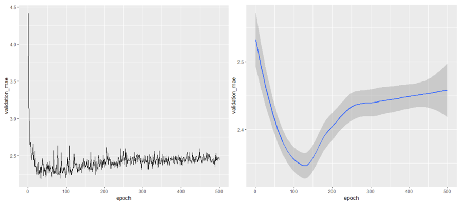
Looking at these plots, we can see that the Validation error rate drop initially as the model is trained. When the number of epochs increases beyond about 125, there is a lot of over-fitting as the validation error increases. So it is best we stop training the model before 125 epochs.
So while training, we will specify epochs = 80 to avoid overfitting.
model <- build_model()

hist = model %>% fit(train_data, train_targets, epochs = 80, batch_size = 16, verbose = 0)
# re-run the code chunks before linear regression model if you get an error
plot(hist)
result <- model %>% evaluate(test_data, test_targets)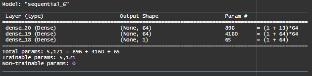
In our Multiple Linear Regression, we had only 7 parameters (5 covariates, 1 intercept and 1 sigma parameter). In our neural network, we have about 5000 parameters !
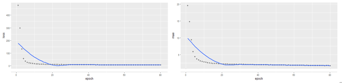
The loss = 16.756 and MAE = 2.617. This means that we are approximately off by $2617 on average. Our Neural Network clearly outperforms the Multiple Linear Regression Model with a 27.96% reduction in Mean Absolute Error.
To Summarise,
| Model | Mean Absolute Error | Predicted Median House prices are … |
|---|---|---|
| Linear Regression | 0.3633 | … off by $3633 on average. |
| Neural Network | 2.617 | … off by $2617 on average. |
A simple neural network was able to outperform the Linear Regression Model. To achieve higher accuracy, we will need more data or explore more complex structured neural networks.